November Recap - Geographic Information Systems
Geographic Information Systems or GIS are specialized technology used for spatial data that require mapping. In our November meetup, R-Ladies Philly member and GIS Specialist Mary Lennon introduced R-Ladies Philly to manipulating and plotting spatial data from our favorite city (Philly!) in our favorite language (R!)!
How can we access and store spatial data?
First, Mary explained that GIS data can be stored in different formats including Shapefiles, GPX, and GeoJSON. In this workshop, we used Shapefile because it is the most commonly used format, and is publically available. Briefly, Shapefiles store the geometric location and attributes of geographic features (e.g. census areas in Philadelphia) based on vector features. Vector features consist of individual points with x/y (latitude/longitude) coordinates that can be joined to create a line or a polygon. Although we did not work with this data type, GIS data can also be stored in ‘raster’ format which plot spatial data as pixels or cells, with each pixel having a specific assigned value.
We worked with two datasets during this workshop:
- Spatial data from tidycensus (available here )
- Tabular data from the publicly-available American Community Survey dataset (ACS), which contains information about the US and its people with known spatial components at national, regional, and local levels.
Using R to represent spatial data visually
We read in spatial data from tidycensus using the rgdal package and plotted it using default settings:
# Read in the shapefile, and see file structure
census_boundaries <- rgdal::readOGR("Census_Boundaries",layer = "cb_2017_42_tract_500k")## OGR data source with driver: ESRI Shapefile
## Source: "/Users/katerinaplacek/Documents/R/RLadies_Philly/spatial/Spatial_Workshop_Data/Census_Boundaries", layer: "cb_2017_42_tract_500k"
## with 3217 features
## It has 9 fields
## Integer64 fields read as strings: ALAND AWATERhead(census_boundaries@data) # here, we focus on the @data slot as it contains the attribute information for the shapefile## STATEFP COUNTYFP TRACTCE AFFGEOID GEOID NAME LSAD
## 0 42 003 020100 1400000US42003020100 42003020100 201 CT
## 1 42 003 051100 1400000US42003051100 42003051100 511 CT
## 2 42 003 070800 1400000US42003070800 42003070800 708 CT
## 3 42 003 080700 1400000US42003080700 42003080700 807 CT
## 4 42 003 130100 1400000US42003130100 42003130100 1301 CT
## 5 42 003 160800 1400000US42003160800 42003160800 1608 CT
## ALAND AWATER
## 0 1678102 483177
## 1 190118 0
## 2 446679 0
## 3 275058 0
## 4 772138 0
## 5 1029321 0plot(census_boundaries) # use default plotting to examine dataIncorporating spatial data with nonspatial data, and other spatial data
Next, we learned to incorporate non-spatial data from ACS with spatial data from tidycensus to aid in geographical distinction between variables pertinent to the Philadelphia community.
We imported and inspected the nonspatial data from ACS:
acs_data <- read.csv('acs_data.csv')head(acs_data)## GEOID NAME
## 1 4.2101e+10 Census Tract 1, Philadelphia County, Pennsylvania
## 2 4.2101e+10 Census Tract 2, Philadelphia County, Pennsylvania
## 3 4.2101e+10 Census Tract 3, Philadelphia County, Pennsylvania
## 4 4.2101e+10 Census Tract 4.01, Philadelphia County, Pennsylvania
## 5 4.2101e+10 Census Tract 4.02, Philadelphia County, Pennsylvania
## 6 4.2101e+10 Census Tract 5, Philadelphia County, Pennsylvania
## variable B08121_001_estimate B08121_001_moe
## 1 B08121_001 63650 9854
## 2 B08121_001 40472 17900
## 3 B08121_001 70300 9533
## 4 B08121_001 54250 7936
## 5 B08121_001 61542 12941
## 6 B08121_001 52625 6852
## Total_Worked_At_Home_estimate Total_Worked_At_Home_021_moe
## 1 106 62
## 2 8 13
## 3 147 63
## 4 162 82
## 5 82 58
## 6 36 21
## Total_Married_Couple_Family_estimate Total_Married_Couple_Family_moe
## 1 511 156
## 2 438 86
## 3 554 114
## 4 465 106
## 5 490 151
## 6 122 39
## Total_PopOneRace_White_estimate Total_PopOneRace_White_moe
## 1 3020 405
## 2 825 271
## 3 2740 323
## 4 1605 210
## 5 2721 417
## 6 1126 231And then merged the nonspatial ACS data with the spatial data from tidycensus by each data point’s GEOID:
# The spatial object needs to be listed first in the merge function for the result to be a spatial object.
acs_spatial <-
  sp::merge(x = census_boundaries, y = acs_data, by = "GEOID")
We then learned how to incorporate spatial data from tidycensus with spatial data from ACS - this is essential for plotting geographically precise datapoints, for instance on a map. Mary emphasized the importance of each dataset’s coordinate reference system, or CRS, for mapping. The CRS specififes ‘where in the world’ your spatial data exists, and can be expressed in different coordinate systems (see espi.io for a reference list of coordinate systems).
To find which CRS your spatial data are stored in, we use the following function and the CRS is listed after “+ellps”; Here, our data are in the GRS80 reference system:
# The ACS spatial data
acs_philly@proj4string## CRS arguments:
## +proj=longlat +datum=NAD83 +no_defs +ellps=GRS80 +towgs84=0,0,0# The Philadelphia county boundary
Phila_County@proj4string## CRS arguments:
## +proj=lcc +lat_1=40.96666666666667 +lat_2=39.93333333333333
## +lat_0=39.33333333333334 +lon_0=-77.75 +x_0=600000.0000000001
## +y_0=0 +datum=NAD83 +units=us-ft +no_defs +ellps=GRS80
## +towgs84=0,0,0Importantly, in order for two datasets to be joined together, they must have the same CRS! In our data, this is the case, but if you needed to change the CRS of your datasets, you can do so using the sp package:
Phila_County <- sp::spTransform(x = Phila_County, CRSobj = WGS84)
acs_spatial <- sp::spTransform(x = acs_spatial, CRSobj = WGS84)
Here, we have put both the Phila_County data from tidycensus and the ACS spatial data in the ‘WGS84’ CRS which is commonly used in GIS.
Once they were in the same CRS, we used raster to join the two datasets:
acs_philly <-
  raster::intersect(Phila_County,
                    acs_spatial)
Now, on to plotting!
Now, with spatial and demographic data from the ACS successfully combined with census information, we can plot different features of Philadelphia.
Here, we plot the medium income for each census tract in the Philadelphia area:
tm_shape(acs_philly) + tm_fill("MedInc_Est", palette = "Reds")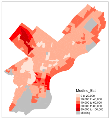
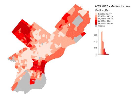
We can further alter the presentation of this data by using built-in features from the tmap package:
tm_shape(acs_philly) +
  #Setting the color and style of the mapping
  tm_fill(
  "MedInc_Est",
  style = "jenks",
  n = 5,
  palette = "Reds",
  legend.hist = TRUE
) +

  #Altering the legend
  tm_layout(
    "ACS 2017 - Median Income",
    legend.title.size = 1,
    legend.text.size = 0.6,
    legend.width = 1.0,
    legend.outside = TRUE,
    legend.bg.color = "white",
    legend.bg.alpha = 0,
    frame = FALSE
  )
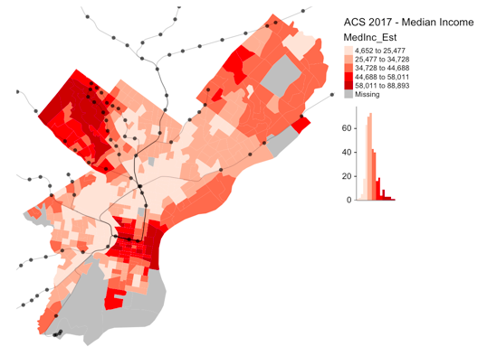
…And we can add in further spatial data from SEPTA to plot ACS data relative to census spatial data AND public transportation access:
tm_shape(acs_philly) +

  #Setting the color and style of the mapping
  tm_fill(
  "MedInc_Est",
  style = "jenks",
  n = 5,
  palette = "Reds",
  legend.hist = TRUE
) +

  #Altering the legend
  tm_layout(
    "ACS 2017 - Median Income",
    legend.title.size = 1,
    legend.text.size = 0.6,
    legend.width = 1.0,
    legend.outside = TRUE,
    legend.bg.color = "white",
    legend.bg.alpha = 0,
    frame = FALSE
  ) +

  #Adding in SEPTA stations and the lines of transport beween them
  tm_shape(SEPTA_RR) +
  tm_lines(col = "black", scale = 1, alpha = 0.25) +
  tm_shape(SEPTA_Staions) +
  tm_dots(
    col = "black",
    scale = 2.5,
    alpha = 0.7,
    shape = 16
  )
For an even more visually-appealing map, we can add in a ‘basemap’ to the background:
tmap_mode("view") # View for interactive

tm_shape(acs_philly) +

  #Setting the color and style of the mapping
  tm_fill(
  "MedInc_Est",
  style = "jenks",
  n = 5,
  palette = "Reds",
  legend.hist = TRUE
) +

  #Altering the legend
  tm_layout(
    "ACS 2017 - Median Income",
    legend.title.size = 1,
    legend.text.size = 0.6,
    legend.width = 1.0,
    legend.outside = TRUE,
    legend.bg.color = "white",
    legend.bg.alpha = 0,
    frame = FALSE
  ) +

  #Adding in SEPTA stations and the lines of transport beween them
  tm_shape(SEPTA_RR) +
  tm_lines(col = "black", scale = 1, alpha = 0.25) +
  tm_shape(SEPTA_Staions) +
  tm_dots(
    col = "black",
    scale = 2.5,
    alpha = 0.7,
    shape = 16
  ) +
  tm_basemap(providers$OpenStreetMap.BlackAndWhite)
And there you have it - an introduction to GIS in R!
Resources
Mary has kindly provided the materials from the November meetup on her github, and she suggests the following spatial datasets if you’re interested in exploring more:
PASDA - Open GIS Data Access for Pennsylvania. Includes a variety of different types of data both raster and vector ranging from centerlines to roads to flood depth grids.
Open Data Philly - A catalog of all the open data in the Philadelphia region (some of which is spatial). The repository covers topics from arts and culture to politics and real-estate.
National Map Viewer - The data download for the National Map Viewer, maintained by the United Staes Geological Survey primarily has land cover and elevation data. This is a good place to get a raster to play with.
Open Government - Open data repository for the US government covering everything from agriculture to maritime and finance.
Thank You Mary, Sponsors, and WeWork!
Many thanks to Mary for leading this informative meetup, to Mica Data Labs and the PENN Masters in Urban Spatial Analytics program for sponsoring delicious pizza and refreshments, and to WeWork for hosting R-Ladies Philly!
This post was authored by Katerina Placek. For more information contact philly@rladies.org